

Architecting any software solution that deals with large amounts of data can present unique challenges, and Endeca implementations are no exception. Understanding the impacts of large data sets to an Endeca implementation and some strategies to handle them can help you better plan for such an undertaking, and in the end, provide a more robust, performant, and maintainable solution.
Architecting the Runtime Environment
Dgraph vs. Agraph
Endeca provides two basic architectures to choose from when implementing an Endeca solution: Dgraph deployment or Agraph deployment.
In a Dgraph deployment, the information for all records in the index is contained within a single set of index files which can be run on a single machine. Even if multiple machines are running the index for load-balancing purposes, they all contain a copy of the same complete index.
By contrast, an Agraph (“A” for “aggregated”) takes a request from a client, sends that request on to multiple Dgraphs running on other machines, aggregates the results, and then sends the aggregated response back to the client. In an Agraph deployment, each of the component Dgraphs contains a different, mutually exclusive portion of the total index data. Agraphs have some minor limitations when compared to Dgraphs, such as the fact that they do not support relevance ranking for dimension search and do not support the Static relevance ranking module. Apart from these specific features and some minor performance degradation, the functionality of an Agraph and Dgraph are the same.
The decision between a Dgraph and Agraph deployment can depend on several factors, but primarily will be driven by the size and nature of your data set. A Dgraph deployment is preferable whenever possible since it is significantly less complex and retains all Endeca’s features. An Agraph deployment can be significantly more complex but can handle larger amounts of data and can more easily grow (by adding additional component Dgraphs) to accommodate increasing amounts of data. The rule of thumb here is to use a Dgraph as long as all your data for the foreseeable future will fit.
Unfortunately, there are no hard and fast rules about how many records or how much data can fit in a single Dgraph. The overall capacity of the Dgraph will be limited by the amount of memory available in your deployment environment, and the amount of memory required by your index will depend heavily on the nature of the data in your index. For instance, if you are indexing metadata only, such as for a large product catalog, you are likely to be able to fit many more records in the same amount of memory than if you are indexing the full text of large document bodies. Since the capacity of a Dgraph is dependent on the available memory, the underlying hardware architecture becomes an important consideration.
32-bit vs. 64-bit
Although some 64-bit system architectures have existed for decades, primarily in supercomputing applications, 32-bit has long been more prevalent, even for production deployment hardware. Recently, however, the availability and software support for 64-bit systems has increased, and the cost has decreased, making this a viable option even for smaller deployments.
One of the primary advantages of a 64-bit architecture over a 32-bit architecture is the memory management. On a 32-bit system, 4GB of memory is the theoretical maximum amount that can be used by the system, and with many operating systems, the limit under real-world conditions can be significantly less that that. On 64-bit systems, however, the theoretical memory ceiling is increased to 16 exabytes (17,179,869,184GB!), roughly 4 billion times the 4GB limit of 32-bit systems. In reality, the potential amount of memory available will be limited by the construction of the physical machine, and how much memory can be installed. Many modern server systems can accommodate 64GB or more, allowing a huge increase in the available memory for running processes.
This is a key advantage in the context of Endeca deployments because it means that many large-scale implementations that would have required an Agraph deployment on 32-bit systems can now be comfortably accommodated by a Dgraph running on a 64-bit system. Once freed from the confines of a 32-bit architecture, it is not at all unreasonable to have a set of index files in the 10’s of gigabytes range or more that can run under a single Dgraph, and this easily allows millions, or even tens of millions of records (again, depending on the data) to be handled within a single Dgraph. When the option of a 64-bit architecture is available, it is a natural choice for an Endeca deployment because of the increased potential capacity.
Note: One of the best approaches to determine the necessary memory requirements for your Dgraph is to build small test Dgraphs with several representative subsets of your data, and determine what the size requirements are for those, then extrapolate your total size requirements from there. For instance, if you can build a Dgraph of 10% of your data that uses 1GB, a Dgraph of 20% of your data uses 2GB, a Dgraph of 30% of your data uses 3GB, etc. it is a reasonable estimate that your entire data will fit in 10-12GB. Depending on how your data changes over time, you may want to consider reserving additional capacity for future growth in the data.
Optimizing Forge
In addition to determining the configuration of the running index or indices, you will need to determine how to most efficiently forge the data; that is, retrieve data from the source system and perform any required processing in preparation for indexing. Just retrieving, not to mention processing, millions of rich records from a source repository might take hours or even days of run time, and the update frequency requirements of your deployment may preclude running a full baseline on a regular basis. There are a number of strategies to consider that can help optimize the forge process.
Note: For clarity, the following discussions are in the context of building a single index for a Dgraph deployment, but can largely be applied to Agraph deployments as well.
General Strategies and Guidelines
There are several guidelines to keep in mind when designing Endeca pipelines that will handle large volumes of data. As the volume of data grows, so does the importance of these considerations, as the effect of any inefficiencies in the pipeline are effectively multiplied by the amount of data the pipeline needs to process. Several key rules to keep in mind are:
- Rule #1: Reduce the amount of extraneous data passed through the pipeline.
- Rule #2: Reduce the number of pipeline components.
- Rule #3: Process data as early in the pipeline as possible.
Consider the following basic pipeline (Dimension flow is excluded for clarity):
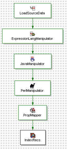
Figure 1:
Figure 1 – Basic Pipeline, Not Optimized
Whenever a record manipulator accesses data in a record, it has to read the entire record into memory, and often, iterate over all the fields that are defined on that record. As a result, any extra data on records, even if it’s never mapped to Endeca properties or dimensions, can slow down the pipeline dramatically. Recall Rule #1: Reduce the amount of extraneous data passed through the pipeline.
The first thing to check is that the LoadSourceData record adapter is only dealing with the data and metadata that will actually be mapped to the Endeca properties and dimensions. For example, if this record source uses a query into a database to retrieve data, make sure only the necessary fields are specified explicitly instead of using a “SELECT *” approach. In some cases it may not be possible to specify the desired fields in the record adapter (if the data comes from a feed previously extracted from a database, for instance). In this case, it is probably advantageous to insert a record manipulator whose job is to remove any unneeded data from the records before they continue through the pipeline.
Since each record manipulator in the pipeline needs to read in each record that is being processed in its entirety, overhead is introduced for each record manipulator that is defined. Reducing the overall number of manipulators by combining multiple manipulators into one will speed the processing time, as well. Recall Rule #2: Reduce the number of pipeline components.
Note: It is also worth noting that the ‘native’ Endeca XML expression language manipulators are significantly faster than Java manipulators, which are, in turn, faster than Perl manipulators. When the choice is available, this should be the order of preference for implementing record manipulators.

Figure 2:
Figure 2 – Basic Pipeline, Optimized
Figure 2 shows the pipeline optimized to reduce the number of manipulators. In this case, the ExpressionLangManipulator should also take care of removing any extraneous data.
In the case of this simplistic pipeline, there is not much choice of where in the pipeline manipulators are placed to perform data processing and cleansing As the complexity of the pipeline increases, the placement of manipulators (Rule #3) will become increasingly important, as you will see in the following sections.
Parallelizing Forge
In many cases, it may be advantageous to split forge into multiple parallel components for harvesting and manipulating the data. This approach can often take advantage of multi-processor and multi-core architectures to reduce the overall processing time, and can be especially beneficial when there is a lot of processing that needs to be done in the Endeca pipeline. However, this approach can also significantly increase the complexity of your forge processes, and should be undertaken only when the performance benefits will outweigh the complexity overhead.
The basic idea is to create multiple ‘component’ forge pipelines that can each harvest and process a portion of the source data, and a ‘merge’ pipeline that can then bring all the resultant records together and prepare them for indexing.
Consider the basic pipeline from Figure 1, above. We could modify that pipeline as follows:
- Remove the
PropMapperProperty Mapper - Remove the
IndexRecsOutput Adapter - Add an Output Record Adapter
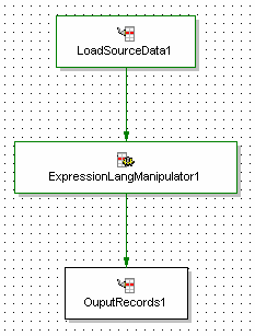
Figure 3:
Figure 3 – Basic Component Pipeline
This pipeline, shown in Figure 3, then becomes one of our ‘component’ pipelines. Instead of performing the property mapping and outputting records prepared for indexing, the pipeline simply outputs the records to a file on the filesystem. Note that you may get a warning from Endeca Developer Studio that this pipeline does not contain a Property Mapper component or an Indexer Adapter component. This is fine, since we are going to perform those tasks in the new ‘merge’ pipeline.
Multiple copies of this pipeline can then be made and adjusted to create the multiple component pipelines as needed. These component pipelines will each process a portion of the records and write the results out to the filesystem, where they can be picked up by the ‘merge’ pipeline.
Figure 4 shows the ‘merge’ pipeline that reads in each of the outputs from the component forges, assembles them, performs the property and dimension mapping, and outputs the records ready to be indexed. Generally a switch join is the appropriate assembler method to use in this scenario. This example shows four components, but you could use more or fewer depending on the capabilities and limitations of your environment. It often makes sense to have one component forge per processor or core in the forge machine, so each forge can have a dedicated processing thread.
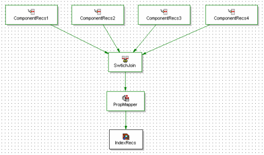
Figure 4:
Figure 4 – Basic Merge Pipeline
Note that the individual component pipelines now need to be configured to retrieve only the records that are appropriate for that component. This may be tricky depending on the number of component forges, and the source of data. It is best to divide the records in a way that is both deterministic and distributes the load evenly. For instance, if the records have an auto-generated ID field you may be able to use that to split them up into buckets, i.e. component 1 handles records whose ID ends in ‘0’, ‘1’, or ‘2’, component 2 handles records whose ID ends in ‘3’, ‘4’, or ‘5’, etc. You may also be able to use other pseudo-random fields such as the millisecond portion of a creation timestamp. If possible, it is best to avoid using fields that may change over time or may not yield an even distribution, such as product, document, or author names.
Notice that the data processing and manipulation is handled in the component pipelines rather than in the merge pipeline. If we had put the ExpressionLangManipulator after the SwitchJoin in the merge pipeline, the eventual output would be the same, but the processing would be significantly slower. Not only would we lose out on the opportunity to parallelize the processing done by that manipulator, but if that manipulator also removes extraneous data as mentioned in the previous section, then we also would be spending unnecessary processing time, memory, and disk I/O handling all that data when writing to disk, reading from disk, and processing the record join. Here you can see Rule #3 from the previous section come into play: Process data as early in the pipeline as possible.
Another advantage of this parallelization scheme is that if for some reason one component forge fails, others may still be able to continue normally, and only the offending component forge may need to be rerun, instead of having to reprocess the entire data set.
Note: If you plan to implement partial updates in conjunction with a parallelized forge, be sure that your partial pipeline contains the appropriate manipulations and mappings that exist both in the component pipelines and the merge pipeline.
Differential Updates
Differential updates are another strategy that can be very effective when dealing with large amounts of data, especially when retrieving records from the source system is expensive, or if only a small portion of that data will be changing at any given time. Be sure not to confuse differential updates as described here with partial updates, where record updates are sent directly to a running MDEX Engine.
Note: Partial updates are another valuable tool that may be useful in your deployment, but are not specifically covered here. For more information on partial updates, see the Endeca ITL Guide
The basic idea of differential updates is to modify the forge pipeline so that only records that have been changed since the last run are harvested and processed. Then those records can be merged with the records gathered on a previous run. This can save a tremendous amount of processing time over retrieving the entire data set on each forge run. All the records are still run through the index process on a regular basis, but this is often fast compared to the time spent harvesting and processing the records initially
There are several conditions that must be met for this strategy to work. The first is that the records in the source system must have a non-volatile unique key or ID field. Secondly, the source system must expose an indication of when a particular record was last updated. If these pieces of information are not available from the source system, there is no way to know which records may be new or updated since the last run. Additionally, the time when the last run occurred must be recorded somewhere accessible to the adapter gathering the updated source data so that it can correctly query the source system for new or updated records
Figure 5 provides an example of a basic differential pipeline. Here, the PreviousProcessedData component reads in the records from the previous forge run, while the LoadUpdatedSourceData component queries the source system for the records that have changed since the previous run. The FirstRecordJoin component uses a First Record Join to merge the records, giving the new records priority over the old. That is, if two records come into the join with the same key, it will use the one from the NewRecordsCache instead of the OldRecordsCache. The record caches must use the unique key property mentioned above for the join to work properly
Then, the OutputRecords record adapter writes out the merged records so that they can be read in again on the next run by the PreviousProcessedData component. Note that this occurs before the PropMapper component. The primary reason for this is that if the property or dimension mappings need to change, the output from previous forge outputs can still be used instead of having to be discarded in favor of a completely fresh baseline
Again, recall Rule #3 from the previous section: Process data as early in the pipeline as possible. The ExpressionLangManipulator should be placed before the join. This way, it only has to act on the smaller number of updated records, instead of having to process the entire data set over and over again on successive runs of the forge process.
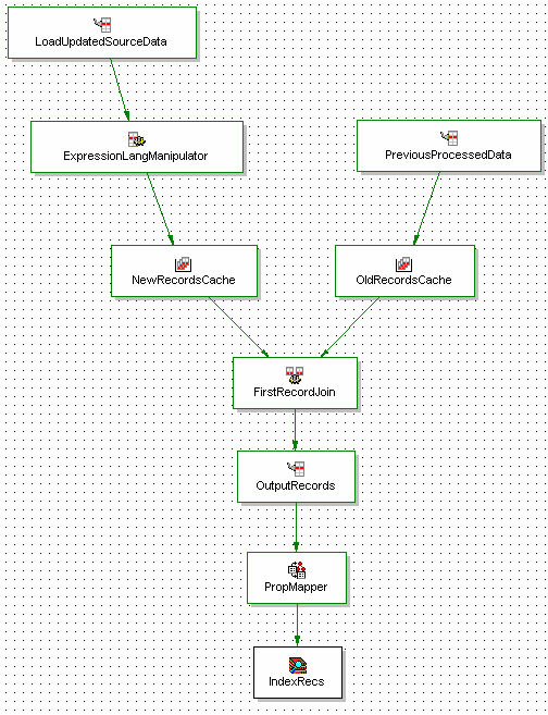
Figure 5:
Figure 5 – Basic Differential Pipeline
One important caveat of the system described here is that it does not handle the case when records are to be removed from the index. There are a couple ways to handle this, depending on the criticality and nature of the record deletions.
If the removal of records from the index is not time-critical, it may be possible to perform periodic complete baselines to remove these records. A complete baseline can be achieved by deleting both the previously gathered data and the indication of when the last forge run occurred. The pipeline will then behave as if it is running for the first time, and will retrieve and process all records from the source system.
If the records are not actually removed, but rather, are ‘logically’ deleted from the source system (marked as ‘hidden’, for instance), then a manipulator placed after the record join can simply remove those records marked for deletion based on the value of the ‘hidden’ flag or other attribute.
If the records are, in fact, deleted from the source system entirely, some complex processing logic would be needed to keep track of which records have been deleted and remove those records from the pipeline accordingly. This would likely require a custom manipulator inserted after the record join that could query the source system to determine which records were to be kept and which were to be deleted.
In some cases, it may even be appropriate to combine the strategies of parallelized forge with differential updates. In this case, each of the component pipelines can be made to accommodate differential processing, and the merge pipeline can handle the record aggregation, property mapping, and preparation for indexing.
Differential updates can also be combined with partial updates, although care must be taken to ensure that the set of data processed by the partial pipeline is in sync with the successive iterations of the differential forge. This generally requires maintaining an external timestamp to indicate to the partial pipeline when the last differential crawl took place.
Conclusion
Although building an Endeca implementation on a data set of millions of records may be daunting, there are some strategies and guidelines that can prove helpful in making it more manageable. I have outlined several in this article:
When architecting a runtime environment,
- Choose a Dgraph over an Agraph as long as your data will fit.
- Choose a 64-bit architecture over a 32-bit architecture when possible, as it makes it much more likely you will be able to fit your entire data into a single Dgraph.
When designing your Endeca pipeline(s),
- Reduce the amount of extraneous data passed through the pipeline.
- Reduce the number of pipeline components.
- Process data as early in the pipeline as possible.
- Consider implementing a parallelized forge when the data requires a significant amount of pipeline processing, and a multi-processor or multi-core system is available.
- Consider implementing differential updates when retrieving data from the source system is expensive or if only a small portion of your source data changes at a time.
I hope this article has provided some helpful guidance towards successful large-scale Endeca deployments. If you have any questions or comments, I encourage you to comment on this article.

